TopoMetry — Multi-Batch Integration
When single-cell datasets are produced in different laboratories, sequencing platforms, or experimental batches, systematic technical differences (“batch effects”) can obscure the underlying biology. Integration methods aim to remove these unwanted technical sources of variation while preserving genuine biological signal.
TopoMetry provides a CCA-anchor integration pipeline (inspired by Seurat v3, Stuart et al. 2019) that corrects batch effects in log-normalised expression space and then builds geometry-aware spectral scaffolds and layouts on the corrected data. Two complementary workflows are supported:
Full integration — correct all batches simultaneously in a single run.
Reference mapping — build a stable reference atlas from a subset of batches, then sequentially map new (query) batches onto it.
In this tutorial you will learn both workflows end-to-end, from quality control to final visualisation and quantitative evaluation.
Dataset: Immune_ALL_human.h5ad from the scIB benchmark (Luecken et al., 2022) — human immune cells across 10 batches and 16 annotated cell types.
Environment & imports
Besides topometry and standard Python libraries, we use scanpy and the AnnData format to manage our single-cell data.
import warnings
warnings.filterwarnings('ignore')

import numpy as np
import scanpy as sc
import anndata as ad
import topo as tp

# figure settings
sc.settings.set_figure_params(dpi=120, facecolor='white', fontsize=14)
sc.settings.verbosity = 1

print(f'scanpy {sc.__version__}  |  topo {tp.__version__}')
scanpy 1.10.3 | topo 1.0.2
Load data
The Immune_ALL_human dataset contains ~33,500 cells from 10 batches spanning multiple tissues and sequencing platforms. The expression matrix is already log-normalised (adata.X), while raw counts are stored in adata.layers['counts']. This is a curated dataset, so we can skip quality-control for demonstration purposes.
You can download the dataset from Figshare.
adata = ad.read_h5ad('Immune_ALL_human.h5ad')

# Create a convenient 'cell_type' alias for the annotation column
adata.obs['cell_type'] = adata.obs['final_annotation'].copy()

print(adata)
print(f"\nBatches   ({adata.obs['batch'].nunique()}): {sorted(adata.obs['batch'].unique())}")
print(f"Cell types ({adata.obs['cell_type'].nunique()}): {sorted(adata.obs['cell_type'].unique())}")
print(f"adata.X max = {adata.X.max():.3f}  (already log-normalised)")
AnnData object with n_obs × n_vars = 33506 × 12303
    obs: 'batch', 'chemistry', 'data_type', 'dpt_pseudotime', 'final_annotation', 'mt_frac', 'n_counts', 'n_genes', 'sample_ID', 'size_factors', 'species', 'study', 'tissue', 'cell_type'
    layers: 'counts'

Batches   (10): ['10X', 'Freytag', 'Oetjen_A', 'Oetjen_P', 'Oetjen_U', 'Sun_sample1_CS', 'Sun_sample2_KC', 'Sun_sample3_TB', 'Sun_sample4_TC', 'Villani']
Cell types (16): ['CD10+ B cells', 'CD14+ Monocytes', 'CD16+ Monocytes', 'CD20+ B cells', 'CD4+ T cells', 'CD8+ T cells', 'Erythrocytes', 'Erythroid progenitors', 'HSPCs', 'Megakaryocyte progenitors', 'Monocyte progenitors', 'Monocyte-derived dendritic cells', 'NK cells', 'NKT cells', 'Plasma cells', 'Plasmacytoid dendritic cells']
adata.X max = 12.041  (already log-normalised)
Workflow 1 — Full integration of all batches
In this workflow we correct all batches simultaneously. This is the simplest approach and works well when you have all your data available upfront.
The pipeline consists of four steps:
prepare_for_integration → run_cca_integration → fit_adata → compute_all_integration_metrics
Prepare data for integration
tp.sc.prepare_for_integration ensures the expression matrix is in the correct format and selects highly variable genes (HVGs) shared across batches — the features that will drive the integration.
Since our data is already log-normalised, we set input_type='lognorm' so no additional normalisation is applied. If you have raw count data, use input_type='counts' instead.
# Work on a copy so the original adata is preserved for Workflow 2
adata_w1 = adata.copy()

tp.sc.prepare_for_integration(
    adata_w1,
    batch_key='batch',
    input_type='lognorm',
    select_hvgs=True,
    n_hvgs=2000,
)

n_feats = len(adata_w1.uns['integration_features'])
print(f"Selected {n_feats} integration features across {adata_w1.obs['batch'].nunique()} batches.")
Selected 2000 integration features across 10 batches.
Run CCA integration
tp.sc.run_cca_integration performs the actual batch correction:
Builds a guide tree to determine the optimal pairwise merge order.
For each merge: computes CCA, finds mutual nearest-neighbour anchors, filters and scores them, and applies a symmetric correction in expression space.
Z-scores the corrected matrix (
scale_output=True) so it is ready fortp.sc.fit_adata.
Key parameters:
n_components=30: number of CCA dimensions (default, same as Seurat).n_jobs=-1: use all available CPU cores for nearest-neighbour searches.
The function returns a new AnnData containing only the integration features.
adata_int = tp.sc.run_cca_integration(
    adata_w1,
    batch_key='batch',
    n_components=30,
    scale_output=True,
    n_jobs=-1,
)

print(adata_int)
AnnData object with n_obs × n_vars = 33506 × 2000
    obs: 'batch', 'chemistry', 'data_type', 'dpt_pseudotime', 'final_annotation', 'mt_frac', 'n_counts', 'n_genes', 'sample_ID', 'size_factors', 'species', 'study', 'tissue', 'cell_type'
    uns: 'cca_integration'
    obsm: 'X_cca'
    varm: 'cca_loadings'
    layers: 'counts', 'lognorm', 'original', 'corrected'
The output AnnData contains:
.X— z-scored corrected expression (ready for TopoMetry).layers['corrected']— corrected log-normalised values.layers['original']— original (uncorrected) values.obsm['X_cca']— CCA coordinates.uns['cca_integration']— integration log (merge order, anchor counts, etc.)
Fit TopoMetry
With the batch-corrected data, we now fit the TopoMetry pipeline — spectral scaffold, refined graphs, 2D layouts, and clustering — using the familiar tp.sc.fit_adata wrapper:
tg_w1 = tp.sc.fit_adata(
    adata_int,
    projections=('MAP'),
    do_leiden=True,
    leiden_resolutions=(0.3,),
    n_jobs=-1,
)

print("Available embeddings:", [k for k in adata_int.obsm.keys()])
2026-03-25 18:37:48.136004: I tensorflow/core/util/util.cc:169] oneDNN custom operations are on. You may see slightly different numerical results due to floating-point round-off errors from different computation orders. To turn them off, set the environment variable `TF_ENABLE_ONEDNN_OPTS=0`.


Available embeddings: ['X_cca', 'X_ms_spectral_scaffold', 'X_spectral_scaffold', 'X_msTopoMAP', 'X_TopoMAP']
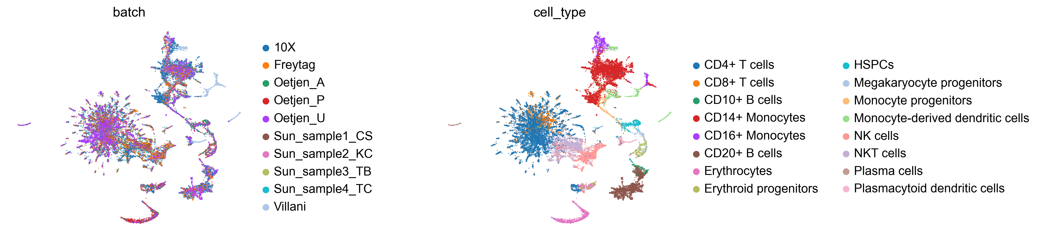
Visualise the integrated embedding
Let’s inspect the TopoMAP layout coloured by batch and cell type. Good integration should show batches well-mixed while preserving cell-type separation:
sc.pl.embedding(adata_int, basis='TopoMAP', color=['batch', 'cell_type'],
                frameon=False, wspace=0.6)
Integration quality metrics
Visual inspection is important, but we also want quantitative measures of integration quality. tp.sc.compute_all_integration_metrics computes six complementary metrics:
Metric |
Measures |
Good integration |
|---|---|---|
kNN purity |
Whether neighbours share the same cell type |
High (close to 1) |
kNN mixing |
Whether neighbours come from different batches |
High (close to 1) |
iLISI |
Local Inverse Simpson Index for batch mixing |
High (up to n_batches) |
cLISI |
Local Inverse Simpson Index for cell-type purity |
Low (close to 1) |
ARI |
Adjusted Rand Index (cluster vs cell-type agreement) |
High (close to 1) |
NMI |
Normalised Mutual Information (cluster vs cell-type) |
High (close to 1) |
We compare the integrated data against an uncorrected baseline (same features, no batch correction):
# Subset original data to the same features for fair comparison
features_w1 = list(adata_int.var_names)
adata_uncorr_w1 = adata_w1[:, features_w1].copy()

metrics_w1 = tp.sc.compute_all_integration_metrics(
    {
        'uncorrected': adata_uncorr_w1,
        'integrated':  adata_int,
    },
    batch_key='batch',
    cell_type_key='cell_type',
    cluster_key='topo_clusters',
    k=100,
    n_jobs=-1,
)

print("=== Workflow 1 — Integration metrics ===")
print(metrics_w1.to_string(float_format='{:.4f}'.format))
=== Workflow 1 — Integration metrics ===
            uncorrected  integrated
knn_purity       0.8202      0.8304
knn_mixing       0.4832      0.6959
ilisi            2.3840      4.6099
clisi            1.1514      1.1022
ari                 NaN      0.5139
nmi                 NaN      0.6430
The iLISI score (batch mixing) should increase substantially after integration, while cLISI (cell-type purity) should remain close to 1 — indicating that batch effects were removed without blurring biological distinctions.
Workflow 2 — Reference atlas + sequential query mapping
In many practical scenarios, you want to build a stable reference atlas and then map new samples onto it — for instance, when new patient cohorts arrive over time, or when you want to annotate new experiments against a well-characterised reference. This workflow supports that use case:
Integrate a subset of batches to build a reference.
Save the reference to disk for re-use.
Prepare held-out query batches.
Find the optimal mapping order (most similar queries first).
Map all queries sequentially.
Fit TopOGraph on the final atlas and evaluate.
prepare_for_integration(ref)  →  run_cca_integration(ref)  →  save_cca_reference
prepare_for_mapping(queries)  →  find_mapping_order  →  map_to_cca_reference
fit_adata(atlas)  →  compute_all_integration_metrics
Define reference and query batches
We use 6 batches as the reference and hold out 4 as queries. In practice, you would choose reference batches that are well-characterised and cover the expected biological diversity:
REF_BATCHES   = ['10X', 'Freytag', 'Oetjen_A', 'Oetjen_P',
                 'Sun_sample1_CS', 'Sun_sample2_KC']
QUERY_BATCHES = ['Oetjen_U', 'Sun_sample3_TB', 'Sun_sample4_TC', 'Villani']

adata_ref_raw = adata[adata.obs['batch'].isin(REF_BATCHES)].copy()
adata_queries_raw = [
    adata[adata.obs['batch'] == b].copy() for b in QUERY_BATCHES
]

print(f"Reference batches ({len(REF_BATCHES)}): {REF_BATCHES}")
print(f"Query batches     ({len(QUERY_BATCHES)}): {QUERY_BATCHES}")
print(f"\nReference cells: {adata_ref_raw.n_obs:,}")
for b, q in zip(QUERY_BATCHES, adata_queries_raw):
    print(f"  Query '{b}': {q.n_obs:,} cells")
Reference batches (6): ['10X', 'Freytag', 'Oetjen_A', 'Oetjen_P', 'Sun_sample1_CS', 'Sun_sample2_KC']
Query batches     (4): ['Oetjen_U', 'Sun_sample3_TB', 'Sun_sample4_TC', 'Villani']

Reference cells: 23,931
  Query 'Oetjen_U': 3,730 cells
  Query 'Sun_sample3_TB': 2,403 cells
  Query 'Sun_sample4_TC': 2,420 cells
  Query 'Villani': 1,022 cells
Prepare and integrate the reference
The reference is prepared and integrated exactly as in Workflow 1:
tp.sc.prepare_for_integration(
    adata_ref_raw,
    batch_key='batch',
    input_type='lognorm',
    select_hvgs=True,
    n_hvgs=2000,
)

print(f"Selected {len(adata_ref_raw.uns['integration_features'])} integration features for the reference.")
Selected 2000 integration features for the reference.
adata_ref = tp.sc.run_cca_integration(
    adata_ref_raw,
    batch_key='batch',
    n_components=30,
    scale_output=True,
    n_jobs=-1,
)

print(f"Reference integrated: {adata_ref.shape[0]:,} cells, {adata_ref.shape[1]} features")
Reference integrated: 23,931 cells, 2000 features
Save and load the reference
A key advantage of this workflow is persistence — you can save the integrated reference to disk and re-use it later without re-running the integration. The CCA loadings and integration metadata are preserved:
REFERENCE_PATH = '/tmp/immune_cca_reference.h5ad'

tp.sc.save_cca_reference(adata_ref, REFERENCE_PATH)
print(f"Reference saved to {REFERENCE_PATH}")

# Demonstrate round-trip: load it back
adata_ref_loaded = tp.sc.load_cca_reference(REFERENCE_PATH)
print(f"Loaded reference: {adata_ref_loaded.shape[0]:,} cells, {adata_ref_loaded.shape[1]} features")
Reference saved to /tmp/immune_cca_reference.h5ad
Loaded reference: 23,931 cells, 2000 features
Prepare query datasets
tp.sc.prepare_for_mapping ensures each query dataset is normalised consistently with the reference and checks feature overlap — how many of the reference’s integration features are present in each query:
tp.sc.prepare_for_mapping(
    adata_queries_raw,
    adata_ref,
    batch_key='batch',
    input_type='lognorm',
)

for b, q in zip(QUERY_BATCHES, adata_queries_raw):
    shared = sum(g in set(adata_ref.var_names) for g in q.var_names)
    print(f"  '{b}': {shared}/{adata_ref.n_vars} reference features covered")
  'Oetjen_U': 2000/2000 reference features covered
  'Sun_sample3_TB': 2000/2000 reference features covered
  'Sun_sample4_TC': 2000/2000 reference features covered
  'Villani': 2000/2000 reference features covered
Find the optimal mapping order
When mapping multiple query batches, it helps to start with the ones most similar to the reference — they contribute the most reliable anchors and produce a more stable atlas. tp.sc.find_mapping_order ranks queries by their CCA similarity to the current reference:
mapping_order = tp.sc.find_mapping_order(
    adata_ref,
    adata_queries_raw,
    n_components=10,
    k=5,
    n_jobs=-1,
)

print("Optimal mapping order (most → least similar to reference):")
for rank, idx in enumerate(mapping_order):
    print(f"  {rank+1}. {QUERY_BATCHES[idx]}")
Optimal mapping order (most → least similar to reference):
  1. Oetjen_U
  2. Sun_sample3_TB
  3. Sun_sample4_TC
  4. Villani
Map queries to the reference
tp.sc.map_to_cca_reference projects each query batch onto the reference, correcting batch effects using the frozen CCA space. Setting return_intermediates=True collects the atlas state after each mapping step — useful for tracking how integration metrics evolve:
adata_atlas, steps = tp.sc.map_to_cca_reference(
    adata_queries_raw,
    adata_ref,
    mode='query_only',
    mapping_order=mapping_order,
    sequential_topometry=False,
    return_intermediates=True,
    n_jobs=-1,
)

print(f"Final atlas: {adata_atlas.shape[0]:,} cells, {adata_atlas.shape[1]} features")
print(f"\nCells per batch:")
print(adata_atlas.obs['batch'].value_counts().to_string())
Final atlas: 33,506 cells, 2000 features

Cells per batch:
batch
10X               10727
Oetjen_U           3730
Freytag            3347
Oetjen_P           3265
Oetjen_A           2586
Sun_sample4_TC     2420
Sun_sample3_TB     2403
Sun_sample2_KC     2281
Sun_sample1_CS     1725
Villani            1022
Fit TopOGraph on the final atlas
With all batches mapped, we fit the full TopoMetry pipeline on the combined atlas:
tg_atlas = tp.sc.fit_adata(
    adata_atlas,
    projections=('MAP'),
    do_leiden=True,
    leiden_resolutions=(0.3,),
    n_jobs=-1,
)

print("Available embeddings:", [k for k in adata_atlas.obsm.keys()])
Available embeddings: ['X_ms_spectral_scaffold', 'X_spectral_scaffold', 'X_msTopoMAP', 'X_TopoMAP']
Visualise the atlas
Let’s inspect the final atlas. We add an origin column to distinguish reference from query cells, then colour by batch, origin, and cell type:
adata_atlas.obs['origin'] = np.where(
    adata_atlas.obs['batch'].isin(REF_BATCHES), 'reference', 'query'
)

sc.pl.embedding(adata_atlas, basis='TopoMAP',
                color=['batch', 'origin', 'cell_type'],
                frameon=False, wspace=0.6)
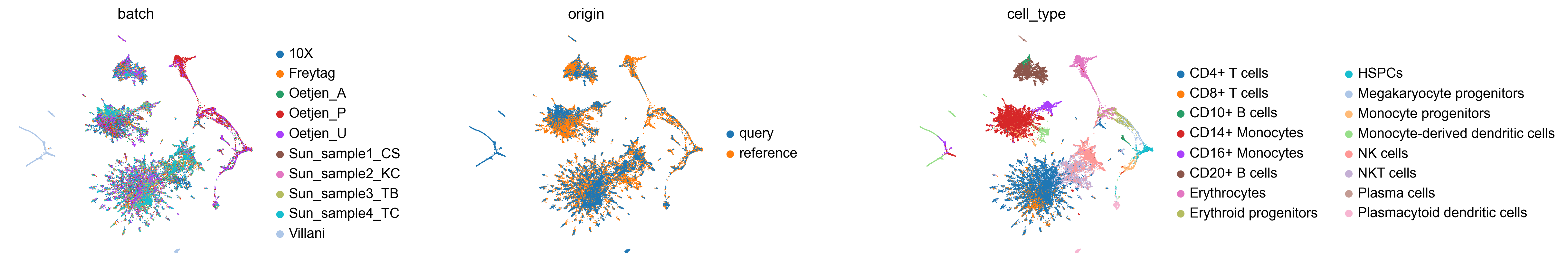
Reference and query cells should overlap for the same cell types, with batches well-mixed within each population.
Integration quality metrics
We build a comprehensive comparison table: uncorrected data, the reference alone, each intermediate mapping step, and the final atlas. This lets us track how batch mixing and cell-type preservation evolve as queries are added:
# Uncorrected baseline: original lognorm data, same features as the reference
features_ref = list(adata_ref.var_names)
adata_uncorr_w2 = adata[:, [g for g in features_ref if g in adata.var_names]].copy()

adata_dict_w2 = {
    'uncorrected': adata_uncorr_w2,
    'reference':   adata_ref,
}

# Add intermediate steps with descriptive labels
for label in sorted(steps.keys()):
    step_idx = int(label.split('_')[1])
    query_name = QUERY_BATCHES[mapping_order[step_idx]]
    adata_dict_w2[f'{label} (+{query_name})'] = steps[label]

adata_dict_w2['final_atlas'] = adata_atlas

metrics_w2 = tp.sc.compute_all_integration_metrics(
    adata_dict_w2,
    batch_key='batch',
    cell_type_key='cell_type',
    cluster_key='topo_clusters',
    k=100,
    n_jobs=-1,
)

print("=== Workflow 2 — Integration metrics ===")
print(metrics_w2.to_string(float_format='{:.4f}'.format))
=== Workflow 2 — Integration metrics ===
            uncorrected  reference  step_0 (+Oetjen_U)  step_1 (+Sun_sample3_TB)  step_2 (+Sun_sample4_TC)  step_3 (+Villani)  final_atlas
knn_purity       0.8191     0.6845              0.6856                    0.6896                    0.6921             0.7201       0.8390
knn_mixing       0.4847     0.8149              0.8413                    0.8542                    0.8653             0.8649       0.6737
ilisi            2.3673     2.7598              2.7811                    2.9519                    3.1464             3.2433       4.0883
clisi            1.1513     1.2424              1.2235                    1.2418                    1.2384             1.1989       1.0991
ari                 NaN        NaN                 NaN                       NaN                       NaN                NaN       0.5467
nmi                 NaN        NaN                 NaN                       NaN                       NaN                NaN       0.6751
As queries are added, iLISI (batch mixing) should increase progressively while cLISI (cell-type purity) remains stable — confirming that the sequential mapping removes batch effects without distorting biology.
Summary
In this tutorial we covered two complementary integration workflows:
Workflow 1 (full integration) |
Workflow 2 (reference mapping) |
|
|---|---|---|
When to use |
All data available upfront |
New batches arrive over time |
API |
|
Same for reference, then |
Reference persistence |
Not applicable |
|
Downstream |
|
Same |
Both workflows use the same underlying CCA-anchor correction. The sequential mapping approach is best suited for incrementally extending a stable reference atlas as new data becomes available.
What’s next?
Explore the Step-by-Step tutorial to learn how to tune individual TopoMetry components.
Use
tp.sc.impute_adata()on the integrated data for denoised gene expression.Apply
tp.sc.evaluate_representations()andtp.sc.plot_riemann_diagnostics()to assess the quality of integrated embeddings.