Evaluating embeddings
As one realizes how much methods and strategies exist for dimensionality reduction, it can be challenging to decide which to use. TopOMetry employs various models, but even so it may be hard to decide for a single one a priori. Instead, a better approach would be to compute several alternatives and score them to decide which to trust more. In this tutorial, we’ll see how to evaluate the results of dimensionality reduction methods.
In TopOMetry, there are three ways to do this quantitatively:
Trustworthiness - this classical score assess the preservation of neighborhoods (i.e., the local structure). It penalizes any unexpected nearest neighbors in the output space, in proportion to their rank in the input space.
Geodesic correlation - this method draws from DEMaP and Heiser and Lau. It estimates the Spearman correlation between geodesic distances in the high- and low-dimensional spaces. This can be very computational expensive and will prioritize isometry (preservation of distances) over isomorphy (preservation of shapes, more related to the trustworthiness score), which is often unbeneficial (e.g., Isomap will by definition have the highest score, but it seldom performs well in preserving geometry). If these terms sound strange, you might want to take a look at the fantastic work on Minimum-Distortion Embedding by Agrawal, Ali and Boyd.
Global score - this draws from the TriMAP paper and is essentially a Minimum Reconstruction Error (MRE) score, normalized by the MRE of PCA (by construction, PCA will have a global score of 1.0).
.
Calculating these metrics can be very insightful when choosing which representations to trust the most. It can also indicate that something went wrong in the learning process (e.g., too small or too large values of k-nearest-neighbors) if you have really low scores. Very rarely a single method will be the best performer in every single score. Instead, there’s usually a tradeoff between preserving distances and preserving geometry, often referred to as the ‘global vs. local’ paradigm. This has been explored by Bohm, Berens and Kobak in neighborhood embeddings.
.
What about qualitative evaluations?
Quantitative evaluations are important for deciding which embedding to trust ‘the most’, but they are not particularly useful to investigate which regions of these embeddings are more worthy of trust than the others. Thus, in addition to these methods, TopOMetry also includes the Riemann metric, which was developed by Perraul-Joncas & Meila in 2013 and had originally been implemented in megaman. It has been adapted into TopOMetry to allow the qualitative evaluation of embeddings and their underlying manifold.
.
For this tutorial, we’ll use a single-cell RNA-seq dataset from the human retina by Lukowski et al., which can be downloaded from CellXGene Datasets as an h5ad file. As usual, we’ll use scanpy to read the file and assist us handling the sc-data.
# Load required libraries:
import numpy as np
import topo as tp
import scanpy as sc
import matplotlib.pyplot as plt
Download the data from CellXGene Datasets. You’ll probably have to generate a new link in their website!
# Grab a new link, CellXGene does not provide permalinks:
#!curl -o retina.h5ad "https://corpora-data-prod.s3.amazonaws.com/10fe0e76-fbae-44d4-a96c-884a416a60b1/local.h5ad?AWSAccessKeyId=ASIATLYQ5N5X42SUPM4X&Signature=PWvopZUW7am79eN%2FkisZWl%2FI90M%3D&x-amz-security-token=IQoJb3JpZ2luX2VjEHgaCXVzLXdlc3QtMiJHMEUCIQCP59wwUyNaFwHZEufQx95hMK56hj%2FoyBng8ivD3E4CkQIgSkLbuhw4UKaKndhllAsSn1oizkyTlr4%2Fz7mzRODEjzgq9AMIwf%2F%2F%2F%2F%2F%2F%2F%2F%2F%2FARABGgwyMzE0MjY4NDY1NzUiDCKWkm3YWbgL3UpMUyrIA8zNOFYUWuWXwOEp%2Fp9ZMdEpumAWyrsuS0Gj2N98ZCvV6OmZbwvj%2FTlN0MF6DOZ%2FA13gp8L5HQEaWym6UR9KmnP%2BDdAkPOSBklVloXYqh9Q6Rg%2FWhEXjYJs9grJJS8mNkukpSppvPz2RSOff08VsCkCGjyAU04zKc9hos6J4PoFXoAeKxgp0e4mwt9MAoYLtjItR40kG1diz4KjY7EZAjmrzY7SlHrxpexLMRoElAOhuu0I9Aj0zNXTIxyO9XpcZK9sTN90ZAuHYMp%2FLR3BuuVrPRmUr9iPpFd8hTRTeIHN5MPnw6u40GUDR0sH%2B5azvmrTNttWLaJnQsq%2BGSXi%2FJdJozeQy6gjHuvOJ1Qd0Mx7%2FHeY6okGj5EUkVeiLDwjzEKtM39GivD5ZvA7vuOgzwSQZbIKcI7HS36kkGza%2FS1xOgYfk1W37RcEzyFToujc6d0CuAj4GrwU9lW%2Fr8x2N%2Bd7GrfLd8hzUFYNPkzToXgfWc7Yr1QZc4emWnESMMNBIlcREisVp%2FARxJ1uWIHjNxnGI3kdSprIydSorim5VDA%2FW3z9p2ms7KfIAIcR0d6t6BGeHB0SqRf22A0ZuPn5r%2BQSGlogd4cZgmzD60ZekBjqlAcDdgleqKBh2pcQHIr50sYkEX9T2Zb161O%2FlUmKhYswS93dacxyETJFhVkiohufV05MItSPU1w9NRQkz91Kd1mbrbgdgFtIQFW9Ry%2FUKK0%2BttCHp36PHQlHe%2FsELthw9qvxtrjQlf2qN87AGvFZGhhN5voiriUFadIJ6Zz24BVT1lUx%2FeajvdtJA9tvecrK3XPrhb70zr0EBVJUb1FrZgMToFhdhgA%3D%3D&Expires=1687120942"
# Load the data:
adata = sc.read_h5ad('retina.h5ad')
It is already preprocessed and has information regarding the highly variable genes (HVG), so we’ll just subset the HVG and perform the standard Z-score transformation:
# Save to raw
adata.raw = adata

# Subset HVG
adata = adata[:, adata.var.highly_variable_features]

# Z score transformation:
sc.pp.scale(adata, max_value=10)
adata
/home/davi/.local/lib/python3.10/site-packages/scanpy/preprocessing/_simple.py:843: UserWarning: Received a view of an AnnData. Making a copy.
  view_to_actual(adata)


AnnData object with n_obs × n_vars = 19694 × 1987
    obs: 'n_genes', 'n_counts', 'percent_mito', 'donor_id', 'assay_ontology_term_id', 'cell_type_ontology_term_id', 'development_stage_ontology_term_id', 'disease_ontology_term_id', 'self_reported_ethnicity_ontology_term_id', 'is_primary_data', 'organism_ontology_term_id', 'sex_ontology_term_id', 'tissue_ontology_term_id', 'author_cell_type', 'suspension_type', 'cell_type', 'assay', 'disease', 'organism', 'sex', 'tissue', 'self_reported_ethnicity', 'development_stage'
    var: 'chromosome', 'featureend', 'featurestart', 'n_cells', 'percent_cells', 'robust', 'highly_variable_features', 'mean', 'var', 'hvf_loess', 'hvf_rank', 'gene_symbols', 'feature_is_filtered', 'feature_name', 'feature_reference', 'feature_biotype', 'std'
    uns: 'cell_type_ontology_term_id_colors', 'default_embedding', 'schema_version', 'title'
    obsm: 'X_diffmap', 'X_diffmap_pca', 'X_fitsne', 'X_fle', 'X_pca', 'X_phi', 'X_umap'
Before we start, we might want to estimate the intrinsic dimensionality of this dataset, to guide the choice of how many eigencomponents to compute:
# Estimate i.d.
from topo.tpgraph import IntrinsicDim

# Initialize the IntrinsicDim class with default parameters:
id_est = IntrinsicDim(
    methods=['fsa','mle'], # the methods we'll use
    k=range(10, 110, 10), # the number of k-neighbors to test
    backend='hnswlib',  # the approximate kNN backend to use
    metric='euclidean', # the distance metric to use
    n_jobs=-1, # the number of jobs to run in parallel
    plot=True, # whether to plot the results during fit()
    random_state=None) # the random state to use for colors

# Estimate the i.d.
id_est.fit(adata.X)
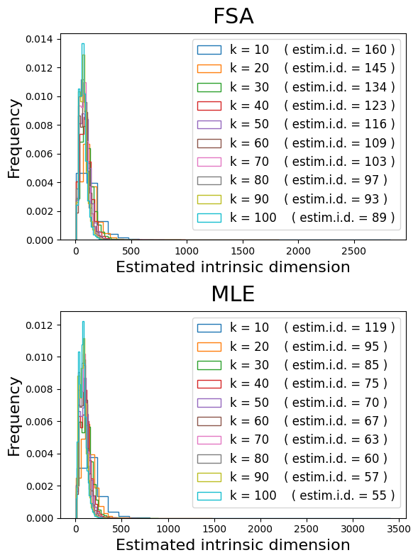
These results suggest we should compute around 150 eigencomponents.
We will also subset the data to only 8,000 cells, for computational tractability (after all, this is only a tutorial):
# Subset the data

sc.pp.subsample(adata, n_obs=8000)
Create a TopOGraph object with the desired parameters, and run some models with it:
# Set up a TopOGraph object:
tg = tp.TopOGraph(n_eigs=150, n_jobs=-1, verbosity=0)

tg.run_models(adata.X, kernels=['bw_adaptive'],
                   eigenmap_methods=['msDM'],
                   projections=['MAP', 'PaCMAP'])
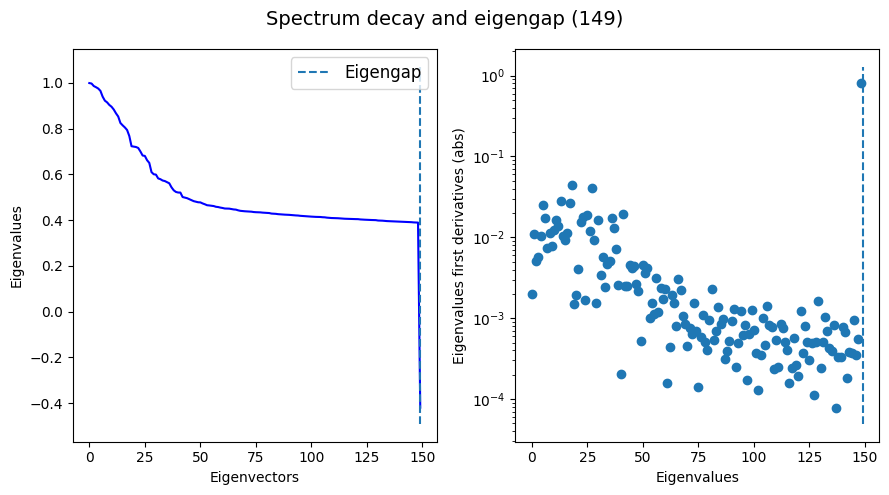
Plot the eigenspectrum to see if we found an eigengap (this is highly desirable).
If an eigengap is not found, we might want to increase the number of eigencomponents we are computing, or to decrease the amount of k-nearest-neighbors in base_knn.
tg.eigenspectrum()
For comparison purposes, we’ll also compute PCA (Principal Component Analysis)…
from sklearn.decomposition import PCA

pca_op = PCA(n_components=150) # compute similar amount of components for fair comparison
pca_Y = pca_op.fit_transform(adata.X)
…and UMAP:
from umap import UMAP

umap_Y = UMAP(n_components=2, metric='cosine').fit_transform(adata.X)
2023-06-14 19:16:37.844537: I tensorflow/core/platform/cpu_feature_guard.cc:182] This TensorFlow binary is optimized to use available CPU instructions in performance-critical operations.
To enable the following instructions: AVX2 FMA, in other operations, rebuild TensorFlow with the appropriate compiler flags.
2023-06-14 19:16:38.576470: W tensorflow/compiler/tf2tensorrt/utils/py_utils.cc:38] TF-TRT Warning: Could not find TensorRT
Before we go on, let’s take a look at our TopOGraph object:
tg
TopOGraph object with 8000 samples and 1987 observations and:
 . Base Kernels:
    bw_adaptive - .BaseKernelDict['bw_adaptive']
 . Eigenbases:
    msDM with bw_adaptive - .EigenbasisDict['msDM with bw_adaptive']
 . Graph Kernels:
    bw_adaptive from msDM with bw_adaptive - .GraphKernelDict['bw_adaptive from msDM with bw_adaptive']
 . Projections:
    MAP of bw_adaptive from msDM with bw_adaptive - .ProjectionDict['MAP of bw_adaptive from msDM with bw_adaptive']
    PaCMAP of msDM with bw_adaptive - .ProjectionDict['PaCMAP of msDM with bw_adaptive']
 Active base kernel  -  .base_kernel
 Active eigenbasis  -  .eigenbasis
 Active graph kernel  -  .graph_kernel
You may have noticed that the naming of representations is quite descriptive within TopOMetry (and hopefully, self-explanatory at some extent). This is to avoid any potential confusion, as several different similarity-learning and matrix decomposition methods may have been used to generate the graphs or eigenbases used for the graph layout optimization. It’s better to know what you are actually doing under the hood, right?!
For clarity, here, we are using
i)the ‘bandwidth adaptive’ kernel method, which is related to the FSA estimate of local intrinsic dimensionality
ii) the multiscale Diffusion Maps eigenmap method
iii) and the MAP and PaCMAP projection methods.
Let’s add these projections to the AnnData object and visualize them, just to know what we’re evaluating:
# Add all embeddings to adata:
adata.obsm['X_pca'] = pca_Y
adata.obsm['X_UMAP'] = umap_Y
adata.obsm['X_topo_msDM'] = tg.EigenbasisDict['msDM with bw_adaptive'].results() # the `results()` method guarantees this is properly weighted
adata.obsm['X_topoMAP'] = tg.ProjectionDict['MAP of bw_adaptive from msDM with bw_adaptive']
adata.obsm['X_topoPaCMAP'] = tg.ProjectionDict['PaCMAP of msDM with bw_adaptive']

# Plot the embeddings:
sc.pl.embedding(adata, basis='pca', color='cell_type')
sc.pl.embedding(adata, basis='UMAP', color='cell_type')
sc.pl.embedding(adata, basis='topo_msDM', color='cell_type')
sc.pl.embedding(adata, basis='topoMAP', color='cell_type')
sc.pl.embedding(adata, basis='topoPaCMAP', color='cell_type')
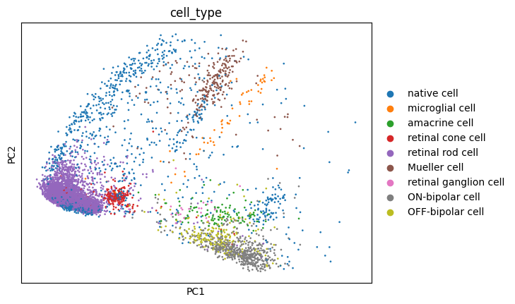
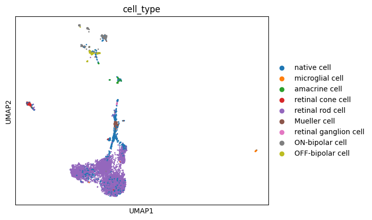
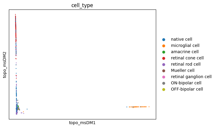
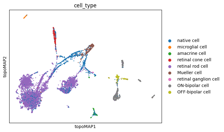
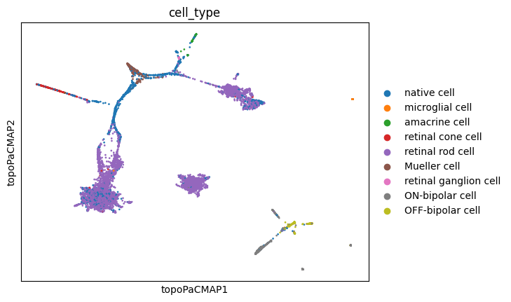
These visualizations make a lot of sense. It is long known that Mueller glia cells can differentiate into retinal rod cells, and thus the continuum of cells between these main cell types is highly indicative of a differentiation trajectory. UMAP, topoMAP and topoPaCMAP, in particular, are highly suggestive of such an underlying biology, although UMAP misses the aparent branching structure.
However, dissecting the cellular hierarchies within this biological system is not our focus here (at this tutorial). Instead, let’s now get started with the quantitative evaluations, at least for the time being:
Quantitative evaluations:
Trustworthiness
This is a very classic metric and is available within scikit-learn. TopOMetry does have an adapted implementation which uses approximate-nearest-neighbors to achieve a better performance, but let’s go with the default scikit-learn one this time.
NOTE: Keep in mind we prefer the cosine metric over the euclidean metric in this case, since the euclidean metric performs very poorly in high-dimensional spaces. You can read the seminal work of Aggarwal, Hinneburg and Keim on it, or go through this recent benchmark for more empirical guidelines.
Also keep in mind that we’ll evaluate the first two dimensions of PCA and UMAP, as we’re interested in the 2-D embeddings in this example. However, we could also compute the scores for the full eigenbasis.
from sklearn.metrics import pairwise_distances
from sklearn.manifold import trustworthiness

# Compute high-dimensional pairwise distances - we'll only need to do this once:
X_dists = pairwise_distances(adata.X, metric='cosine')

# Compute the trustworthiness of each embedding:
print('PCA trustworthiness: ', trustworthiness(X_dists, pca_Y[:,0:2], metric='precomputed'))
print('msDM (topometry) trustworthiness: ', trustworthiness(X_dists, tg.EigenbasisDict['msDM with bw_adaptive'].results()[:,0:2], metric='precomputed'))
print('UMAP (on data) trustworthiness: ', trustworthiness(X_dists, umap_Y, metric='precomputed'))
print('TopoMAP (MAP on diff. graph of msDM) trustworthiness: ', trustworthiness(X_dists, tg.ProjectionDict['MAP of bw_adaptive from msDM with bw_adaptive'], metric='precomputed'))
print('TopoPaCMAP (PaCMAP on msDM) trustworthiness: ', trustworthiness(X_dists, tg.ProjectionDict['PaCMAP of msDM with bw_adaptive'], metric='precomputed'))
PCA trustworthiness:  0.8327973160660661
msDM (topometry) trustworthiness:  0.8335538976476476
UMAP (on data) trustworthiness:  0.8797553115615615
TopoMAP (MAP on diff. graph of msDM) trustworthiness:  0.8950652902902902
TopoPaCMAP (PaCMAP on msDM) trustworthiness:  0.8923884040290291
As we can see, trustworthiness scores can be insightful!
In this case, it points that the local geometry is somewhat equally preserved by topoMAP, topoPaCMAP and UMAP. PCA and msDM also perform very similar in 2 dimensions.
However, this does not tell us much about the global preservation of geometry. The geodesic correlation score is better suited for this.
Before we move on to geodesic correlation, let’s see how we can use TopOMetry to calculate trustworthiness a little faster than with scikit-learn. This involves parallelization, so it escalates well with larger datasets. Let’s compute the trustworthiness of the full PCA and msDM eigenbases:
# Compute the trustworthiness of each embedding:
from topo.eval.local_scores import trustworthiness as tw

print('PCA trustworthiness: ', tw(X_dists, pca_Y, X_is_distance=True))
print('msDM (topometry) trustworthiness: ', tw(X_dists, tg.EigenbasisDict['msDM with bw_adaptive'].results(), X_is_distance=True))
PCA trustworthiness:  0.8997163696060038
msDM (topometry) trustworthiness:  0.9524821763602251
As we can see, the diffusion maps preserve more local geometry than PCA. However, this was largely expected, as PCA cannot handle non-linear structure, which is commonly the case of local geometries in high-dimensional manifolds underlying single-cell datasets. PCA scores tend to get significantly lower as the data becomes increasingly non-linear.
Geodesic correlation
In essence, the geodesic correlation (GC) score computes the Spearman R correlation between geodesic distances in the original high-dimensional data and the learned low-dimensional embedding. It is implemented as a stand-alone function in tp.eval.geodesic_correlation.
Note that this will take significantly longer than computing trustworthiness, and can be rather impractical for larger, real-world datasets. In my laptop this takes about 3min to run (remember we subset the data).
# Compute the GC of each embedding:
print('PCA GC: ', tp.eval.geodesic_correlation(tg.base_knn_graph, pca_Y[:,0:2], metric='euclidean'))

print('msDM (topometry) geodesic correlation: ', tp.eval.geodesic_correlation(tg.base_knn_graph, tg.EigenbasisDict['msDM with bw_adaptive'].results()[:,0:2]))

print('UMAP (on data) geodesic correlation: ', tp.eval.geodesic_correlation(tg.base_knn_graph, umap_Y, metric='euclidean'))

print('TopoMAP (MAP on diff. graph of msDM) geodesic correlation: ', tp.eval.geodesic_correlation(tg.base_knn_graph, tg.ProjectionDict['MAP of bw_adaptive from msDM with bw_adaptive']))

print('TopoPaCMAP (PaCMAP on msDM) geodesic correlation: ', tp.eval.geodesic_correlation(tg.base_knn_graph, tg.ProjectionDict['PaCMAP of msDM with bw_adaptive']))
PCA GC:  0.7117563717324723
msDM (topometry) geodesic correlation:  0.7614853273575543
UMAP (on data) geodesic correlation:  0.7607284605143158
TopoMAP (MAP on diff. graph of msDM) geodesic correlation:  0.5735511990282101
TopoPaCMAP (PaCMAP on msDM) geodesic correlation:  0.4655048730535026
The geodesic correlation score shows that msDM preserves the most of intercellular distances, followed by UMAP, and then PCA.
It is noticeable that the topoMAP and topoPaCMAP we computed performed rather poorly in this evaluation for this particular dataset.
Let’s use this example as an exercise to guide tuning hyperparameters of MAP (‘UMAP on a diet’) and PaCMAP. We could also systematically optimize them using scikit-learn (since all TopOMetry classes are scikit-learn transformers and can be pipelined). However, for the sake of brevity, let’s just recompute them with less iterations and then recalculate the GC scores:
new_topomap = tg.project(projection_method='MAP',
                        num_iters=300, #default 500

)

new_topopacmap = tg.project(projection_method='PaCMAP',
                        num_iters=300, #default 500
)
Now recalculate the GC scores:
print('New TopoMAP (MAP on diff. graph of msDM) GC: ', tp.eval.geodesic_correlation(tg.base_knn_graph, new_topomap, metric='euclidean', n_jobs=-1, backend='hnswlib'))

print('New TopoPaCMAP (PaCMAP on msDM) GC: ', tp.eval.geodesic_correlation(tg.base_knn_graph, new_topopacmap, metric='euclidean', n_jobs=-1, backend='hnswlib'))
New TopoMAP (MAP on diff. graph of msDM) GC:  0.7313449688377016
New TopoPaCMAP (PaCMAP on msDM) GC:  0.4782383856188254
So we actually increased their GC scores by tuning these hyperparameters! Yay!
But have we lost geometry by doing this? (Remember the isometry/isomorphy trade-off !) Let’s check by recalculating the trustworthiness:
print('TopoMAP (MAP on diff. graph of msDM) trustworthiness: ', trustworthiness(X_dists, new_topomap, metric='precomputed'))
print('TopoPaCMAP (PaCMAP on msDM) trustworthiness: ', trustworthiness(X_dists, new_topopacmap, metric='precomputed'))
TopoMAP (MAP on diff. graph of msDM) trustworthiness:  0.8926969187937938
TopoPaCMAP (PaCMAP on msDM) trustworthiness:  0.8939261574074074
According to these two scores, these layouts are now much better than they were before! We have increased their isometrism (i.e. the preservation of distances, related to the GC score) without sacrificing much isomorphism (i.e. the preservation of neighborhoods, related to the trustworthiness score).
Note that we did that without actually looking at them! - this is rather important to avoid confirmation biases (e.g. tuning hyperparameters until it ‘looks good’). We’ll do it now, knowing that these embeddings are at least supposed to be better than before:
adata.obsm['topoMAP_new'] = new_topomap
adata.obsm['topoPaCMAP_new'] = new_topopacmap

sc.pl.embedding(adata, basis='topoMAP_new', color='cell_type')
sc.pl.embedding(adata, basis='topoPaCMAP_new', color='cell_type')
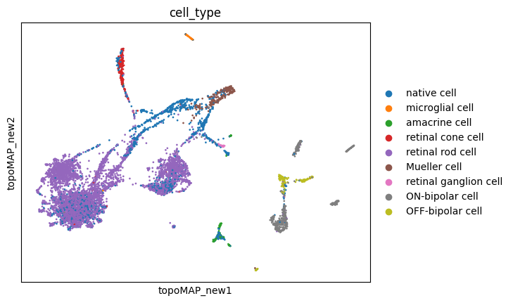
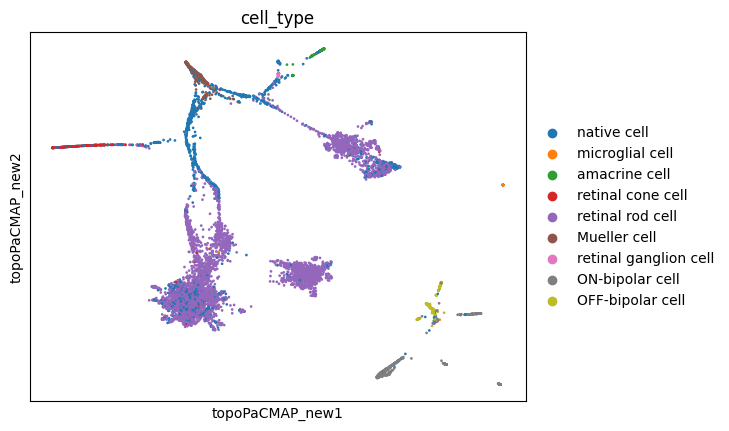
These new embeddings indeed seem much more representative of a developmental cellular lineage, with some branchings included! Let’s hold this thought for a while.
Global score
We can also compute the global score for each embedding. The global score is a rough measurement of how well the projection can reconstruct the original dataset (from a global perspective). It is defined as the normalized mean reconstruction error (MRE). Because PCA has the smallest MRE’s by construction, we use its MRE as a normalization factor. As such, we won’t bother computing it here.
from topo.eval.global_scores import global_score_pca

print('msDM (topometry) global score: ', global_score_pca(adata.X, tg.EigenbasisDict['msDM with bw_adaptive'].results()[:,0:2]))
print('UMAP (on data) global score: ', global_score_pca(adata.X, umap_Y))
print('TopoMAP (MAP on diff. graph of msDM) global score: ', global_score_pca(adata.X, tg.ProjectionDict['MAP of bw_adaptive from msDM with bw_adaptive']))
print('TopoPaCMAP (PaCMAP on msDM) global score: ', global_score_pca(adata.X, tg.ProjectionDict['PaCMAP of msDM with bw_adaptive']))
print('TopoMAP (new) (MAP on diff. graph of msDM) global score: ', global_score_pca(adata.X, new_topomap))
print('TopoPaCMAP (new) (PaCMAP on msDM) global score: ', global_score_pca(adata.X, new_topopacmap))
msDM (topometry) global score:  0.945782912013318
UMAP (on data) global score:  0.9717562
TopoMAP (MAP on diff. graph of msDM) global score:  0.97268474
TopoPaCMAP (PaCMAP on msDM) global score:  0.94945097
TopoMAP (new) (MAP on diff. graph of msDM) global score:  0.97268474
TopoPaCMAP (new) (PaCMAP on msDM) global score:  0.94945097
Because TopOMetry uses a similar spectral initialization to that used in UMAP, these embeddings actually preserve most of the global structure of the data. This is in line with some really cool work from Kobak and Linderman.
As such, we care much more with preserving the local structure of the data (isomorphic and isometric), as the global structure can be taken for granted, given an appropriate initialization for the graph layout optimization step.
Quantitative one-liner
Pufff, these evaluations involve are a lot of analyses, right?
To make it easier, TopOMetry allows users to execute all these analyses with a single one-liner. The results are then stored in a dictionary of dictionaries, each containing one quantitative metric.
Here it is with the default parameters and some explanation on them. You won’t need all of this if you’re running by yourself, but do check the API do make sure you’re doing what you actually aim to.
# Recommended: remove verbosity - this function outputs a lot of text
tg.verbosity = 0

evaluation_dict = tp.pipes.eval_models_layouts(tg, adata.X,
                        kernels=['bw_adaptive'], # kernels to use (there are the three main ones)
                        eigenmap_methods=['msDM','DM','LE'], # eigenmap methods to use
                        projections=['MAP', 'PaCMAP'], # projections to use
                        additional_eigenbases=None, # additional eigenbases to use (e.g. VAEs)
                        additional_projections={'UMAP':umap_Y, 'topoMAP_adjusted': new_topomap, 'topoPaCMAP_adjusted':new_topopacmap}, # additional projections to use (e.g. VAEs, UMAP, UMAP on PCA)
                        n_neighbors=3, # How many neighbors to consider during trustworthiness and GC
                        n_pcs=100, # How many PCs to evaluate in PCA (30 evaluated by default)
                        n_jobs=-1  # How many threads to use (the neighborhood search and GC are highly parallelizable)
                        )
Now print the resulting dict:
evaluation_dict
{'Eigenbasis - Trustworthiness': {'msDM with bw_adaptive': 0.8098173702313947,
'DM with bw_adaptive': 0.7974199395455492,
'LE with bw_adaptive': 0.7626712268084219,
'PCA': 0.7451636725543194},
'Eigenbasis - Geodesic correlation': {'msDM with bw_adaptive': 0.8005793713208497,
'DM with bw_adaptive': 0.49514602567054955,
'LE with bw_adaptive': 0.16496323691989606,
'PCA': 0.8315193212381643},
'Eigenbasis - Global score': {'msDM with bw_adaptive': 0.8042626766730079,
'DM with bw_adaptive': 0.8569706381982813,
'LE with bw_adaptive': 0.8601076061216947},
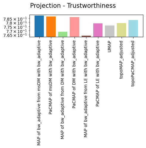
'Projection - Trustworthiness': {'MAP of bw_adaptive from msDM with bw_adaptive': 0.788199223473004,
'PaCMAP of msDM with bw_adaptive': 0.7873825411715656,
'MAP of bw_adaptive from DM with bw_adaptive': 0.768284756097561,
'PaCMAP of DM with bw_adaptive': 0.7863778820095892,
'MAP of bw_adaptive from LE with bw_adaptive': 0.7636725609756098,
'PaCMAP of LE with bw_adaptive': 0.7785516885553471,
'UMAP': 0.7761680008171475,
'topoMAP_adjusted': 0.7789213872650701,
'topoPaCMAP_adjusted': 0.7828817660862823},
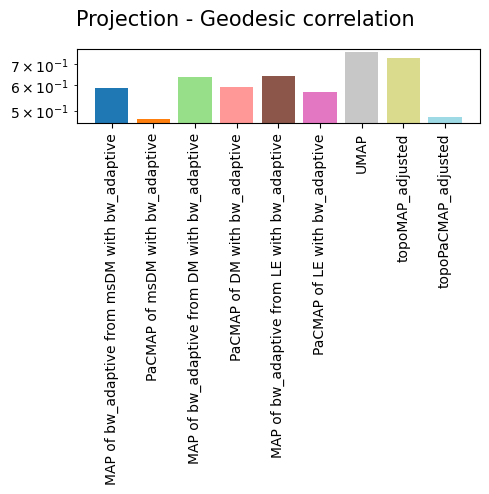
'Projection - Geodesic correlation': {'MAP of bw_adaptive from msDM with bw_adaptive': 0.5893330782558539,
'PaCMAP of msDM with bw_adaptive': 0.4698259111749053,
'MAP of bw_adaptive from DM with bw_adaptive': 0.6370707263954517,
'PaCMAP of DM with bw_adaptive': 0.5910339598972394,
'MAP of bw_adaptive from LE with bw_adaptive': 0.6417686842328263,
'PaCMAP of LE with bw_adaptive': 0.5698940494749563,
'UMAP': 0.7602956642112844,
'topoMAP_adjusted': 0.7313449688377016,
'topoPaCMAP_adjusted': 0.4782383856188254},
'Projection - Global score': {'MAP of bw_adaptive from msDM with bw_adaptive': 0.9722521,
'PaCMAP of msDM with bw_adaptive': 0.94781697,
'MAP of bw_adaptive from DM with bw_adaptive': 0.96429235,
'PaCMAP of DM with bw_adaptive': 0.94446146,
'MAP of bw_adaptive from LE with bw_adaptive': 0.9693363,
'PaCMAP of LE with bw_adaptive': 0.96341056,
'UMAP': 0.9717562,
'topoMAP_adjusted': 0.97268474,
'topoPaCMAP_adjusted': 0.94945097}}
TopOMetry also has a convenience function to allow users to plot all of these quality metrics. Note that here we are using a log scale to make the differences more visible!
tp.pl.plot_all_scores(evaluation_dict, fontsize=10, figsize=(5,5), log=True)
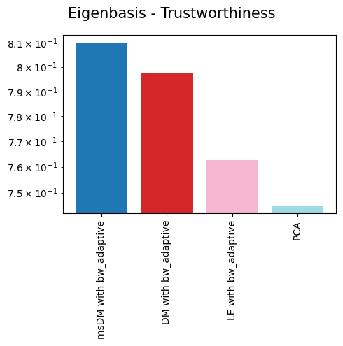
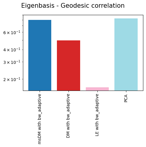
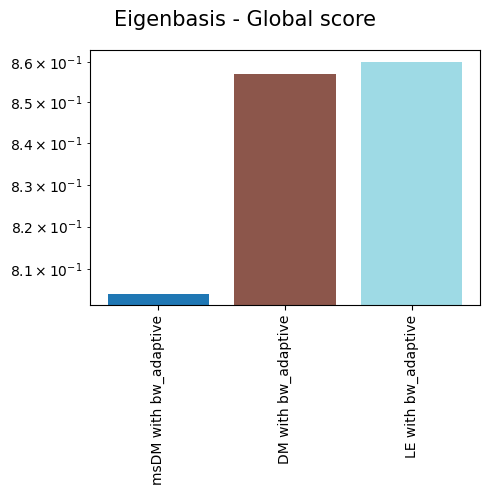
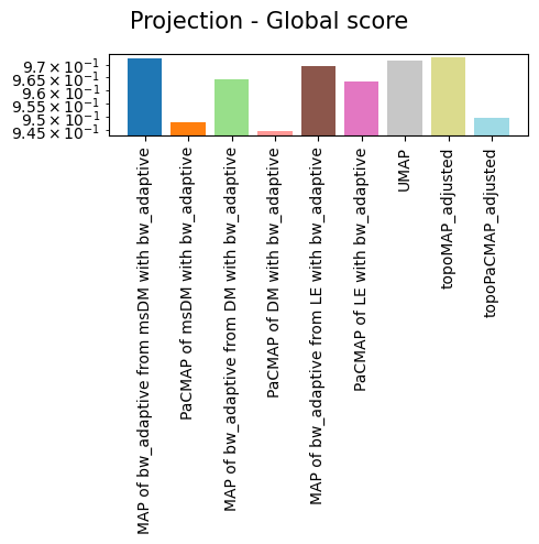
As we can see, non-linear eigenbases perform better than PCA in preserving the local geometry (isomorphism, represented by the trustworthiness score) and distances between cells (isometrism, represented by the geodesic correlation score). The cost for this is a lower preservation of global structure (represented by the global score), although they are not much worse than PCA in that regard.
Regarding the projections, it is easy to see that no single projection scores first in all metrics, but all of them preserve most of the global structure. This is largely expected, as per the Kobak and Lindermann report, the initialization will dictate whether or not a graph layout sucessfully preserves the global structure. More important than that is the preservation of geometry and distances, in which TopOMetry models outperform UMAP.
Qualitative evaluation with the Riemannian metric
Based on these previous quantitative evaluations, one may claim that the ‘topoMAP’ is the best representation for this dataset (technically MAP of the diffusion potential kernel built from the bandwidth adaptive kernel on top of the multiscale diffusion map obtained with the same kernel - but you got the idea), although UMAP can also be a contender due to its high GC score.
This is fine - however, what about different regions within a single embedding (e.g. topoMAP)?
.
Can we be sure that all cells were homogenously embedded with no preferential distortion happening to any celltypes? - You guessed right, we can’t! At least not a priori.
.
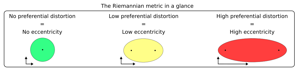
To solve this issue, we need to discover which regions of the manifold are preferentially distorted, and in which directions. This can be qualitatively done by using the Riemannian metric. In a nuthshell, visualizing the Riemannian metric allows one to define how much of the underlying data topology is being preserved by the low-dimensional visualization - in that sense, it augments visualizations by informing in which direction distortions ocurred.
.
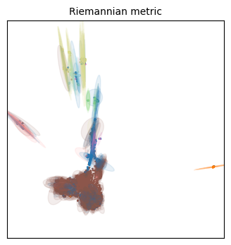
We visualize the Riemannian metric with ellipses. If no distortion ocurred at all during the embedding, the ellipse will have zero eccentricity (i.e. it will be a circle). If distortion ocurred preferentially at one direction, the axis of the ellipse will be elongated along that direction (i.e. it will have a higher eccentricity). Keep in mind this only works in two dimensions!
Quantifying this eccentricity allows us to add this information to the AnnData object to check if any cell types are preferentially distorted.
For starters, we’ll need a graph Laplacian - in this case, we’ll use the default normalized graph Laplacian computed by the Kernel class within the TopOGraph.
NOTE: You can revisit the anatomy of a TopOGraph object at the ‘TopOMetry at a glance’ image in the ‘About TopOMetry’ tab.
# Get the graph Laplacian of our base graph kernel:
L = tg.base_kernel.L
# Define how many ellipses to plot:
n_plot = 1000
# Convert the labels to integers:
labels = adata.obs['cell_type'].cat.codes
# Name the projections you want to plot:
projections = ['UMAP', 'topoMAP', 'topoPaCMAP']
# Plot the Riemann metric
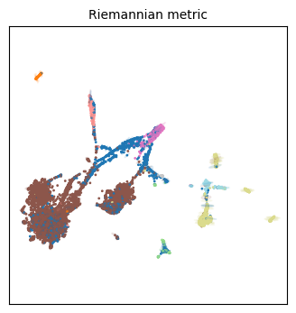
for name in projections:
xy_coord = adata.obsm['X_' + name]
tp.pl.plot_riemann_metric(xy_coord, # The coordinates of the projection
L, # The graph Laplacian
std=0.5, # A scaling factor for the ellipses size
n_plot=n_plot, # How many ellipses to plot
labels=labels,
cmap='tab20', # For coloring
random_state=tg.random_state, # For coloring
figsize=(4,4) # Size of the figure (NEEDS TO BE SQUARE!!!)
)
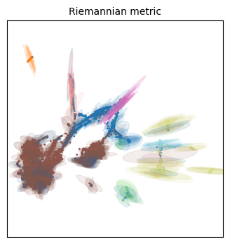
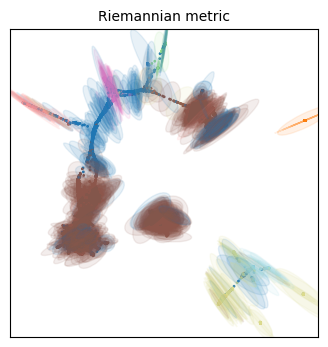
Unfortunately we have different colors from our original embeddings, but we can work with this!
Qualitatively speaking, all three embeddings have more distortion on the cellular populations that are situated on its periphery. This makes some sense, as they will be forced away from dissimilar populations, but everything will still have to fit the 2D place, so the most numerous (i.e. frequent/common) populations are expected to have less distortion.
Right now these are not particularly insightful. To help, we can change the base radius to improve our visualization by changing the parameter std. If it is too large or too small, the visualization will not be particularly useful. Let’s take a closer look at the ‘topoMAP’ embedding, varying the scaling factor std.
tp.pl.plot_riemann_metric(adata.obsm['X_topoMAP'], L, std=0.1, n_plot=n_plot, labels=labels, cmap='tab20', random_state=tg.random_state,  figsize=(4,4))
tp.pl.plot_riemann_metric(adata.obsm['X_topoMAP'], L, std=0.3, n_plot=n_plot, labels=labels, cmap='tab20', random_state=tg.random_state,  figsize=(4,4))
tp.pl.plot_riemann_metric(adata.obsm['X_topoMAP'], L, std=0.5, n_plot=n_plot, labels=labels, cmap='tab20', random_state=tg.random_state,  figsize=(4,4))
<Axes: title={'center': 'Riemannian metric'}>
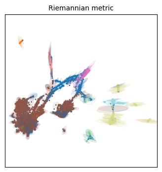
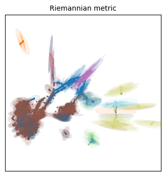
Indeed our ‘periphery hypothesis’ seems to be compatible to these visualizations, particularly as the scaling factor increases. All ellipses on the periphery point toward the center, meaning the distances have been distorted to be bigger in these elongated directions than they would actually be in the high-dimensional manifold. It means we should be careful when interpreting these ‘distances’ as a sign of actual dissimilarity.
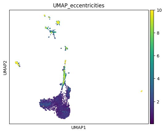
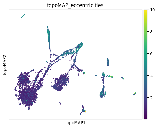
To try to obtain further insights, we can also quantify and color-code the eccentricity of these ellipses to have a better insight on which neighborhoods/celltypes are being preferentially distorted, and then add thee information back to our AnnData object:
# the `get_eccentricity` functions calculates ellipses eccentricity using the Riemann metric
from topo.utils import get_eccentricity

# Create an empty dictionary to store the eccentricities:
eccentricities = {}

for name in projections:
    xy_coord = adata.obsm['X_' + name]
    eccentricities[name] = get_eccentricity(xy_coord, L)

adata.obs['UMAP_eccentricities'] = eccentricities['UMAP']
adata.obs['topoMAP_eccentricities'] = eccentricities['topoMAP']
adata.obs['topoPaCMAP_eccentricities'] = eccentricities['topoPaCMAP']
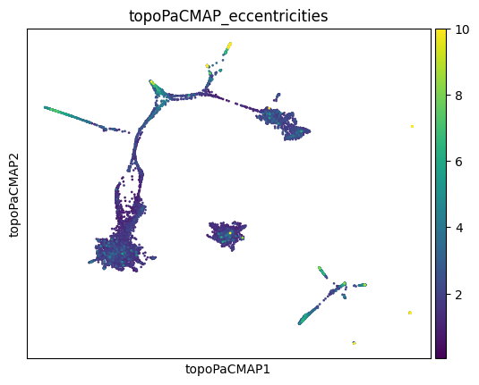
And now we can plot this information just as we would with any other metadata in scanpy! We’ll set a vmax to help us visualize it better.
sc.pl.embedding(adata, basis='UMAP', color='UMAP_eccentricities', vmax=10)
sc.pl.embedding(adata, basis='topoMAP', color='topoMAP_eccentricities', vmax=10)
sc.pl.embedding(adata, basis='topoPaCMAP', color='topoPaCMAP_eccentricities', vmax=10)
We can also visualize this as a violin plot, grouping by cell types:
We can also quantify and color-code the eccentricity of these ellipses to have a better insight on which neighborhoods/celltypes are being preferentially distorted, and then add thee information back to our AnnData object:
fig, (ax1, ax2, ax3) = plt.subplots(1, 3, figsize=(14, 4))
ax1 = sc.pl.violin(adata, 'UMAP_eccentricities', groupby='cell_type', rotation = 80, ylabel=None, ax=ax1, show=False,log=False, scale='area', fontsize=10, ncol=1)
ax1.set_title('UMAP', fontsize=14)
ax1.set_ylabel('')
ax1.set_ylim(bottom=0,top=20)

ax2 = sc.pl.violin(adata, 'topoMAP_eccentricities', groupby='cell_type', rotation = 80, ylabel=None, ax=ax2, show=False,log=False, scale='area', fontsize=10, ncol=1)
ax2.set_title('TopOMetry MAP\n on msDM diff. potential', fontsize=14)
ax2.set_ylabel('')
ax2.set_ylim(bottom=0,top=20)

ax3 = sc.pl.violin(adata, 'topoPaCMAP_eccentricities', groupby='cell_type', rotation = 80, ylabel=None, ax=ax3, show=False,log=False, scale='area', fontsize=10, ncol=1)
ax3.set_title('TopOMetry PaCMAP \n on msDM', fontsize=14)
ax3.set_ylabel('')
ax3.set_ylim(bottom=0,top=100)
(0.0, 100.0)
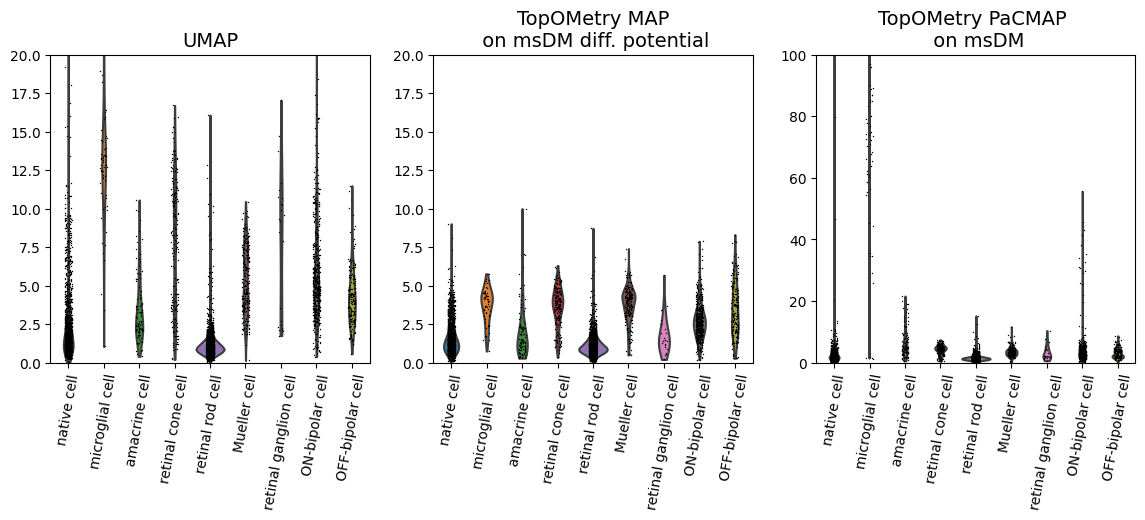
As we can see, some populations are more distorted than others, and this varies across different embeddings. If you are making strong considerations about one of these populations, you might want to check them to see if they are more distorted than others in your embedding, or look for an embedding in which they are less distorted.
.
In this case, TopOMetry’s PaCMAP on msDM has quite strong distortions on microglial cells and native cells. topoMAP, on the other hand, seems to have less distortion for the majority of the populations. UMAP is a middle ground in this case.
.
Naturally, we could change the axes limits, plot the ellipses only for these cells and so forth to further investigate this biological system, but that would go far beyond the scope of this tutorial.
Concluding remarks
Evaluating embeddings is central to get reliable results. Unfortunately, such rigor is not usually seen in single-cell applications, and practitioners either tune their UMAPs until they ‘look good’ or use other methods that as variable as UMAP without its formal guarantees.
I hope this really stresses out the need to evaluate several different representations before choosing one of them to use in analyses that are going to guide years of work! There are several other ways to evaluate embeddings, but these are the most direct, computationally efficient and intrinsically related to geometrical properties I could come up with. I do hope they are helpful for your work - if such, please cite TopOMetry.
Feel free to drop a comment on the Issues section or by email if you would like to see different metrics or evaluation approaches here! :)